Deep Sequence Modelling (RNN)
Lesson 2From static networks to time-aware models
Adding memory so networks understand order, not just values
From static networks to time-aware models, adding memory for order
In the previous section, we established the importance of modeling sequential dependencies. We now turn to how the field historically addressed this problem, beginning with a shift from traditional feedforward architectures to networks capable of handling temporal dynamics.
Revisiting the perceptron
Recall the building block from the Perceptron lesson: a perceptron takes a fixed-length input vector, applies a weighted sum, and passes it through a nonlinearity.
Vector form
ϕ, activation · wi, b, learnable parameters
It operates on a single time slice
STATIC SINGLE STEP
with no notion of time or order, which makes it insufficient for sequential data.
Applying feedforward networks to time series: a naive attempt
One naive way to apply a static neural network to sequence data is to treat each time step independently. Imagine rotating our input-output diagram vertically, where each input xt is processed by the same network f to yield an output yt. We repeat this process across all time steps t = 0, 1, 2, …
While this allows us to handle sequences of inputs, each prediction yt is based only on the corresponding xt. There is no memory of what happened at earlier time steps, so it can't model dependencies across time. When predicting a word, the words that came before are crucial; ignoring them cripples the model. This independence assumption contradicts the very premise of sequential modeling, that prior context informs future states.
Introducing recurrence: capturing temporal dependencies
To solve this problem, we introduce a core idea: maintain and update an internal state as the network processes each time step. Let us define this hidden or internal state as ht. At each time step t, we compute:
An updated internal state ht, which is a function of both the current input xt and the previous state ht−1.
An output prediction yt, which now depends on ht rather than directly on xt alone.
This represents how the output at time step t is computed. The output is computed using the current hidden state.
| Symbol | Meaning |
|---|---|
| xt | The input at time step t. For example, a word in a sentence or a stock price at time t. |
| ht−1 | The hidden state from the previous time step (t−1). Think of this as the memory of the RNN. |
| ht | The updated hidden state at time t. |
| f | A function that combines xt and ht−1. This is usually a neural network layer with non-linearity (like tanh or ReLU). |
| yt | The output at time t, computed using the current hidden state. |
| g | A function (often a linear layer followed by softmax, sigmoid, or identity depending on task). |
yt = g(ht), the output at step t is produced from what the RNN "knows" at t (ht), not from xt in isolation.
This setup provides a recurrence relation. The internal state acts as a form of memory, encoding information from past inputs and making it available to influence future computations. Crucially, this creates a dependency chain over time. The prediction at time step t indirectly depends on all inputs x₀, x₁, …, xt seen so far.
This structure defines a Recurrent Neural Network (RNN).
Visualizing recurrence
There are two primary ways to visualize an RNN:
Neurons with recurrence
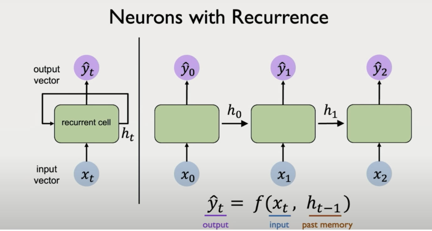
Unrolled view
[Breakdown the RNN into simple blocks of states]
We unroll the recurrence over time. Each time step is shown as a separate copy of the same neural unit, connected to the previous and next states via the hidden variable h.
Useful for backpropagation through time and dependencies between states.
Cyclic view
[Recurrence Relation just like a simple fibonacci function]
We represent the recurrent computation as a loop in the computational graph, the hidden state feeds back into itself over time.
ht−1 → f → ht
feedback along timeEmphasizes structural recurrence, not the full timeline at once.
Both views are functionally equivalent but offer different insights. The unrolled view emphasizes temporal flow. The cyclic view emphasizes structural recurrence.
Step through the recurrence yourself, toggle between unrolled and cyclic views and watch the hidden state evolve. The same W_xh, W_hh, and b_h are reused at every timestep; that's the recurrence insight made concrete:
One cell, reused at every timestep
That's recurrence: a single function f with one fixed set of weights, applied repeatedly across time. As you step forward, the input xt changes and the hidden state ht evolves — but the cell itself is the same one, replicated five times.
Shared weights
Same values at every timestep
W_xh
W_hh
b_h
x1
h1
x2
h2
x3
h3
x4
h4
ht = tanh(Wxh · xt + Whh · ht−1 + bh)
The orange terms are the same at every timestep. Only xt and ht−1 differ.
Why this matters
The introduction of recurrence was a turning point in sequence modeling. It allowed neural networks to:
Learn patterns that span multiple time steps.
Maintain a form of short-term memory.
Generalize across sequences of different lengths using a shared set of parameters.
Although vanilla RNNs are limited in their ability to capture long-term dependencies due to issues like vanishing gradients, they laid the foundation for more advanced architectures such as LSTMs, GRUs, and eventually Transformers.
[Static to Time Aware]
This transition from static to dynamic, time-aware models marked the beginning of deep learning's foray into language, speech, and many other sequence-intensive domains.
Check your understanding
1 / 7The core RNN recurrence is h_t = f(x_t, h_{t-1}). What does h_{t-1} represent?
Practice it yourself
Feel the difference memory makes — the no-state baseline, the shared-weight budget, and the recurrence unrolled. Real Python, hidden tests, no setup.