Deep Sequence Modelling (RNN)

Lesson 3

RNN internal mechanics

The hidden state, recurrence equations, and formal structure

Now that we have an intuitive foundation for recurrent neural networks (RNNs), let us formalize their internal structure and operational semantics. This section builds upon our understanding of the perceptron, the idea of recurrence, and the motivation behind modeling sequences through memory-aware architectures.

Recurrence relations in RNNs

At the heart of an RNN lies the internal state h_t, which is updated as the network processes the input sequence step by step. The update to this state is defined by a recurrence relation, which incorporates both the current input x_t and the prior hidden state h_t−1. This recurrence relation enables the model to retain and evolve a memory of the sequence it has observed so far.

RNN cell & recurrence relation

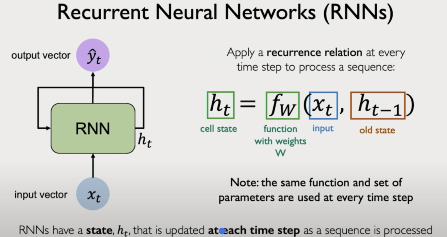
RNN diagram with input x sub t, output y-hat sub t, hidden state loop h sub t, and recurrence h sub t equals f_W of x sub t and h sub t minus 1; same weights each step

The state update can be formally described as:

\mathbf{h}_t = \sigma\!\left( \mathbf{W}_{xh}\mathbf{x}_t + \mathbf{W}_{hh}\mathbf{h}_{t-1} + \mathbf{b}_h \right)

\mathbf{y}_t = \mathbf{W}_{hy}\mathbf{h}_t + \mathbf{b}_y

Symbol	Role
W_xh	weight matrix mapping input to hidden state
W_hh	recurrent weight matrix mapping previous state to current state
W_hy	output weight matrix mapping hidden state to predicted output
σ	element-wise nonlinearity (e.g., tanh or sigmoid), tanh outputs values between −1 and 1, while sigmoid outputs between 0 and 1.
b_h, b_y	bias terms

Weight sharing

These same weight matrices are shared across all time steps, which enforces temporal consistency and greatly reduces the number of trainable parameters.

RNN logic through pseudocode

To further solidify this idea, consider a simple pseudocode example that illustrates how an RNN operates over a sequence:

Python

# Initialize RNN hidden state
h = 0
# Input sequence of words
sentence = ["I", "love", "recurrent", "neural"]
# RNN loop over time
for word in sentence:
    h = update_hidden_state(x=word, h_prev=h)
    y_hat = predict_output(h)

In this code snippet, each word in the input sequence is processed one at a time. The RNN uses the current word and the previously computed hidden state to compute a new hidden state. This new state is then used to produce an output prediction. The process is iterative and maintains a memory of the sequence through the hidden state updates.

word+h_prev→update → h→ŷ

We can visualize the RNN in two complementary ways:

Cyclic form

A looped computation graph where the hidden state is fed back into itself.

Unrolled form

A sequence of computations unwrapped across time, the same operations applied at each time step.

In the unrolled representation:

Aspect	What happens
Inputs	The sequence x₁, x₂, …, x_T flows across time steps.
Hidden state	h_t at each time is passed forward.
Outputs	y_t is generated at each step.
Parameters	The same W_xh, W_hh, W_hy at every time step, weight sharing for variable length and fewer parameters.

Walk through the full forward pass below, stage by stage, timestep by timestep. Every matrix multiply is computed live; every value shown is the real arithmetic.

Inside the RNN cell · stage by stage

Five operations make up one RNN timestep: read input → project via W_xh → add the recurrent term via W_hh → squash with tanh → emit output via W_hy. Watch each stage with real arithmetic.

Stage:→→→→

Timestep:

Stage 1 · Read x_t

The sequence feeds in one timestep at a time

x_1

x_1 ∈ ℝ^3

t = 1 · stage 1/5Speed800ms

Defining loss over time

Training an RNN requires defining a loss function that quantifies the error between predicted and actual outputs. Unlike static models, where a single loss is computed, RNNs compute a loss at each time step. The total loss across a sequence is then the sum of the losses at individual steps:

\mathcal{L}_{\text{total}} = \sum_{t=1}^{T} \mathcal{L}(\hat{\mathbf{y}}_t, \mathbf{y}_t)

This loss drives learning through Backpropagation Through Time (BPTT), where gradients are computed not only over network layers but also across time steps.

Implementation in code

Let us now translate this conceptual understanding into a more explicit code-level implementation.

Consider defining an RNN from scratch using an object-oriented approach:

Python

class SimpleRNN:
    def __init__(self, input_dim, hidden_dim, output_dim):
        self.W_xh = initialize_weights(input_dim, hidden_dim)
        self.W_hh = initialize_weights(hidden_dim, hidden_dim)
        self.W_hy = initialize_weights(hidden_dim, output_dim)
        self.b_h = initialize_bias(hidden_dim)
        self.b_y = initialize_bias(output_dim)
    def forward(self, input_sequence):
        h = np.zeros(self.hidden_dim)
        outputs = []
        for x_t in input_sequence:
            h = activation(np.dot(x_t, self.W_xh) + np.dot(h, self.W_hh) + self.b_h)
            y_hat = np.dot(h, self.W_hy) + self.b_y
            outputs.append(y_hat)
        return outputs

This class encapsulates:

Initialization of weights and biases

Forward pass through the sequence, updating hidden states

Prediction generation at each step

This procedural design closely mirrors the theoretical recurrence structure discussed earlier. It also forms the basis for understanding more complex implementations in TensorFlow or PyTorch.

Run it yourself

Press Run to execute a real SimpleRNN forward pass over a 3-step sequence. The same W_xh, W_hh, W_hy are reused at every step, that's the recurrence:

Python

import numpy as np

np.random.seed(0)

class SimpleRNN:
  def __init__(self, input_dim, hidden_dim, output_dim):
      self.hidden_dim = hidden_dim
      self.W_xh = np.random.randn(input_dim, hidden_dim) * 0.3
      self.W_hh = np.random.randn(hidden_dim, hidden_dim) * 0.3
      self.W_hy = np.random.randn(hidden_dim, output_dim) * 0.3
      self.b_h = np.zeros(hidden_dim)
      self.b_y = np.zeros(output_dim)

def forward(self, input_sequence):
      h = np.zeros(self.hidden_dim)
      outputs = []
      for x_t in input_sequence:
          h = np.tanh(x_t @ self.W_xh + h @ self.W_hh + self.b_h)   # same weights every step
          y_hat = h @ self.W_hy + self.b_y
          outputs.append(y_hat)
      return outputs, h

rnn = SimpleRNN(input_dim=3, hidden_dim=4, output_dim=2)
seq = [np.array([1.0, 0.0, -1.0]), np.array([0.5, 0.5, 0.0]), np.array([-1.0, 1.0, 0.5])]
outputs, h_final = rnn.forward(seq)
for t, y in enumerate(outputs):
  print(f"t={t}  y_hat={np.round(y, 3)}")
print("final hidden state:", np.round(h_final, 3))
print("\nW_hh is reused at every step -> parameter count is independent of sequence length")

First run loads the Python runtime (~10 MB) — takes ~5–10 seconds. Subsequent runs are instant.

From scratch to frameworks

Once you understand the fundamentals of how an RNN functions internally, you can transition to using high-level abstractions in frameworks such as TensorFlow and PyTorch. Both offer RNN modules and layers that encapsulate the forward pass, weight sharing, and even support for batching and sequence padding.

You will practice this in the upcoming lab, where you will implement RNNs for next-word prediction, character generation, and many-to-many sequence classification tasks.

Applications and broader impact

Understanding and building RNNs from scratch equips you to solve sequence-modeling problems across the many-to-one, one-to-many, and many-to-many settings (Lesson 1).

This last setting, many-to-many modeling, is foundational to how large language models function today. Although modern architectures such as Transformers have largely replaced vanilla RNNs due to their scalability and parallelism, the core concepts of sequence modeling, memory, and recurrence remain essential.

Check your understanding

1 / 8

The vanilla RNN hidden-state update is h_t = σ(W_xh · x_t + W_hh · h_{t-1} + b_h). What is the role of W_hh?

Practice it yourself

Build the RNN's machinery — the readout, the loss over time, and the full forward pass. Real Python, hidden tests, no setup.

Project the hidden stateEasy

yₜ = W_hy hₜ + b_y — the readout from memory to prediction.

Loss over timeEasy

Sum the per-step losses — what BPTT pushes back through every step.

SimpleRNN forwardMedium

The whole loop: hidden update + readout, outputs at every step.

RNN internal mechanics

Recurrence relations in RNNs

RNN logic through pseudocode

Unrolled representation and weight sharing

Defining loss over time

Implementation in code

Run it yourself

From scratch to frameworks

Applications and broader impact

Practice it yourself